The Simplex Method

The Simplex method can be used to solve problems of maximizing or minimizing a linear function of variables, with constraints in the form of equalities or inequalities of linear functions of those variables, and with all variables dimensioned above or below

Applying the following steps:

1. Statement of the problem in standard form
2. Application of the Simplex algorithm
3. Determination of the solution obtained

Step 1: Approach the problem as standard

1. The function should be set to "minimize"
2. If necessary, variable changes are made so that all variables have 0 as the lower dimension (X_i\geq 0, \forall i)
3. The restrictions are put with the constant term positive
4. Become the inequalities of the constraints into equalities by adding the slack variables
5. Artificial variables are added to constraints that do not have a variable at the base, and the sum of those artificial variables multiplied by M (which is considered with a very high value) is added to the target function.
6. The table is populated to apply the Simplex algorithm. Its structure is as follows:
   

   	X_1 \cdots X_n
   X basic	to	b
   	c-z

   X_1 \cdots X_n is the alignment of the original variables, slack variables and artificial variables

   to are the terms of such variables in the constraints

   b are the constant elements of such constraints (on the other side of variables in equality)

   c - z are marginal costs, where c are the coefficients of the target function, and z_i=c_{b_1}\cdot a_{1 j}+\cdots+c_{b_m}\cdot a_{m i}, with m being the number of constraints (of elements at the base), and where c_{b_j} represents the coefficient of the target function corresponding to the variable j-th of which they make up the base. Notice that c - z = 0 always for the variables of the base

Step 2: Applying the Simplex Algorithm

1. Election of the column of pivot
   Looking for the lowest element of the row c - z, c\cdot k - z\cdot k among those who are negative and have a positive element in the column a_k. If there is none the algorithm is terminated
2. Choice of the row of pivot
   Among the positive elements of a_k looking for the one with the minimum coefficient: \frac{b_i}{a_{i k}}, we'll call it a_{r k}, and that will be the element on which we will pivot. If there are several with the same coefficient you choose any one
3. Gaussian elimination
   It pivots on a_{r k}, that is, it becomes a_k in a vector of the canonical base. To do this, first divide all the terms in row r from a to a_{r k}, so the new a_{r k} will have a value of 1 (by dividing it between itself). The other elements of the a_k Gaussian elimination (to each i row, with i \not= r, are added the new row r multiplied by X_k). With this the variable -a_{i k} entered the base (and will be located in row r)
4. Repeat
   Until (c_j - z_j\geq 0, \forall j) \cup (a_k < 0, \forall k\longrightarrow c_k - z_k < 0)

Step 3: Determining the solution obtained

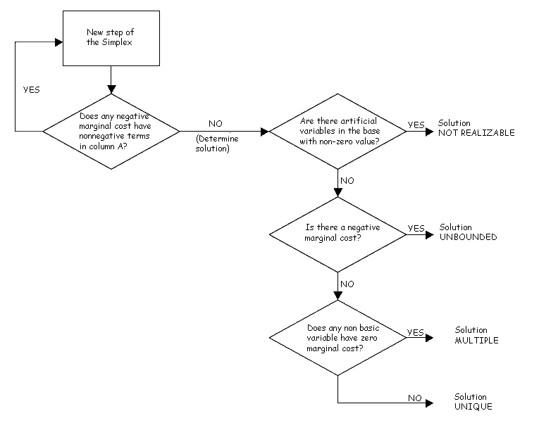
If the problem has artificial variables and some of them have nonzero value in the final solution, then the problem raised has no solution (not feasible). Otherwise, move on to the following cases:

1. If (c_j - z_j\geq 0, \forall j) \cap (c_k - z_ k > 0) for the variables not basic then we have unique solution
2. If (c_j - z_j\geq 0, \forall j) \cap (c_k - z_k = 0) for any variable is not basic then we have multiple solutions
3. If \exists (c_k - z_k < 0) (all of them must comply that a_k < 0) then we have an unstepped solution

Example of problem of the Simplex Method

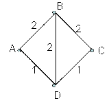
The chart shows the representation of a communication network in which each segment represents the maximum capacity of transfer per unit of time

It is requested to:

1. It proposes a PPL (linear programming problem) whose solution gives us the maximum transfer capacity between A and B and between C and D (the sum of both)
2. Solve the PPL (linear programming problem), indicating the type of solution it is, its value, if there is a solution, and explain it

Part a)

Between A and B there are 3 paths that are:

\begin{cases} X_1 \text{ by the way }A-B \\ X_2 \text{ by the way }A-D-B \\ X_3 \text{ by the way }A-D-C-B \end{cases}

Between C and D there are 3 paths that are:

\begin{cases} X_4 \text{ by the way }C-B-A-D \\ X_5 \text{ by the way }C-B-D \\ X_6 \text{ by the way }C-D \end{cases}

Therefore the function to be optimized is:

(X_1+X_2+X_3)+(X_4+X_5+X_6)

With restrictions:

\begin{cases} X_1+X_4 \leq 2 \\ X_2+X_3+X_4 \leq 1 \\ X_3+X_4+X_5 \leq 2 \\ X_2+X_5 \leq 2 \\ X_3+X_6 \leq 1 \end{cases}

With X_1, X_2, X_3, X_4, X_5, X_6 > 0

Part b)

Maximize (X_1+X_2+X_3)+(X_4+X_5+X_6)
Minimize (-X_1-X_2-X_3)+(-X_4-X_5-X_6)

\begin{cases} X_1+X_4+h_1 = 2 \\ X_2+X_3+X_4+h_2 = 1 \\ X_3+X_4+X_5+h_3 = 2 \\ X_2+X_5+h_4 = 2 \\ X_3+X_6+h_5 = 1 \end{cases}

Values c - z:
column \tiny X_1 = -1 - ( (-1) \cdot 1 + 0 \cdot 0 + 0 \cdot 0 + 0 \cdot 0 + (-1) \cdot 0 ) = 0
column \tiny X_2 = -1 - ( (-1) \cdot 0 + 0 \cdot 1 + 0 \cdot 0 + 0 \cdot 1 + (-1) \cdot 0 ) = -1
column \tiny X_3 = -1 - ( (-1) \cdot 0 + 0 \cdot 1 + 0 \cdot 1 + 0 \cdot 0 + (-1) \cdot 1 ) = 0
column \tiny X_4 = -1 - ( (-1) \cdot 1 + 0 \cdot 1 + 0 \cdot 1 + 0 \cdot 0 + (-1) \cdot 0 ) = 0
column \tiny X_5 = -1 - ( (-1) \cdot 0 + 0 \cdot 0 + 0 \cdot 1 + 0 \cdot 1 + (-1) \cdot 0 ) = -1
column \tiny X_6 = -1 - ( (-1) \cdot 0 + 0 \cdot 0 + 0 \cdot 0 + 0 \cdot 0 + (-1) \cdot 1 ) = 0
column \tiny h_1 = 0 - ( (-1) \cdot 1 + 0 \cdot 0 + 0 \cdot 0 + 0 \cdot 0 + (-1) \cdot 0 ) = 1
column \tiny h_2 = 0 - ( (-1) \cdot 0 + 0 \cdot 1+ 0 \cdot 0 + 0 \cdot 0 + (-1) \cdot 0 ) = 0
column \tiny h3 = 0 - ( (-1) \cdot 0 + 0 \cdot 0 + 0 \cdot 1 + 0 \cdot 0 + (-1) \cdot 0 ) = 0
column \tiny h4 = 0 - ( (-1) \cdot 0 + 0 \cdot 0 + 0 \cdot 0 + 0 \cdot 1 + (-1) \cdot 0 ) = 0
column \tiny h5 = 0 - ( (-1) \cdot 0 + 0 \cdot 0 + 0 \cdot 0 + 0 \cdot 0 + (-1) \cdot 1 ) = 1

\tiny{\begin{pmatrix}& -1\hspace{1 mm} X_1& -1\hspace{1 mm} X_2& -1\hspace{1 mm} X_3& -1\hspace{1 mm} X_4& -1\hspace{1 mm} X_5& -1\hspace{1 mm} X_6& 0\hspace{1 mm} h_1& 0\hspace{1 mm} h_2& 0\hspace{1 mm} h_3& 0\hspace{1 mm} h_4& 0\hspace{1 mm} h_5& \cr -1\hspace{1 mm} X_1& 1& 0& 0& 1& 0& 0& 1& 0& 0& 0& 0& 2 \cr 0\hspace{1 mm} h_2& 0& 1& 1& 1& 0& 0& 0& 1& 0& 0& 0& 1 \cr 0\hspace{1 mm} h_3& 0& 0& 1& 1& 1& 0& 0& 0& 1& 0& 0& 2 \cr 0\hspace{1 mm} h_4& 0& 1& 0& 0& 1& 0& 0& 0& 0& 1& 0& 2 \cr -1\hspace{1 mm} X_6& 0& 0& 1& 0& 0& 1& 0& 0& 0& 0& 1& 1 \cr & 0& -1& 0& 0& -1& 0& 1& 0& 0& 0& 1&\end{pmatrix}}

We chose row 2, column 2, as pivot. So in this case \frac{b_i}{a_{i k}} it will be \frac{1}{1}=1

\tiny{\begin{pmatrix}& -1\hspace{1 mm} X_1& -1\hspace{1 mm} X_2& -1\hspace{1 mm} X_3& -1\hspace{1 mm} X_4& -1\hspace{1 mm} X_5& -1\hspace{1 mm} X_6& 0\hspace{1 mm} h_1& 0\hspace{1 mm} h_2& 0\hspace{1 mm} h_3& 0\hspace{1 mm} h_4& 0\hspace{1 mm} h_5& \cr -1\hspace{1 mm} X_1& 1& 0& 0& 1& 0& 0& 1& 0& 0& 0& 0& 2 \cr 0\hspace{1 mm} X_2& 0& 1& 1& 1& 0& 0& 0& 1& 0& 0& 0& 1 \cr 0\hspace{1 mm} h_3& 0& 0& 1& 1& 1& 0& 0& 0& 1& 0& 0& 2 \cr 0\hspace{1 mm} h_4& 0& 0& -1& -1& 1& 0& 0& -1& 0& 1& 0& 1 \cr -1\hspace{1 mm} X_6& 0& 0& 1& 0& 0& 1& 0& 0& 0& 0& 1& 1 \cr & 0& 0& 1& 1& -1& 0& 1& 1& 0& 0& -1& 1\end{pmatrix}}

We chose row 4, column 5, as pivot. So in this case \frac{b_i}{a_{i k}} it will be \frac{1}{1}=1

\tiny{\begin{pmatrix}& -1\hspace{1 mm} X_1& -1\hspace{1 mm} X_2& -1\hspace{1 mm} X_3& -1\hspace{1 mm} X_4& -1\hspace{1 mm} X_5& -1\hspace{1 mm} X_6& 0\hspace{1 mm} h_1& 0\hspace{1 mm} h_2& 0\hspace{1 mm} h_3& 0\hspace{1 mm} h_4& 0\hspace{1 mm} h_5& \cr -1\hspace{1 mm} X_1& 1& 0& 0& 1& 0& 0& 1& 0& 0& 0& 0& 2 \cr 0\hspace{1 mm} h_2& 0& 1& 1& 1& 0& 0& 0& 1& 0& 0& 0& 1 \cr 0\hspace{1 mm} h_3& 0& 0& 2& 2& 0& 0& 0& 1& 1& -1& 0& 1 \cr 0\hspace{1 mm} X_5& 0& 0& -1& -1& 1& 0& 0& -1& 0& 1& 0& 1 \cr -1\hspace{1 mm} X_6& 0& 0& 1& 0& 0& 1& 0& 0& 0& 0& 1& 1 \cr & 0& 0& 0& 0& 0& 0& 1& 0& 0& 1& -1& 2\end{pmatrix}}

Since there are no more negative values in c – z, c_k - z_k that we can pivot, we stop the algorithm and we get the following result:

\begin{cases} X_1 = 2 \\ X_2 = 1 \\ X_5 = 1 \\ X_6 = 1 \end{cases}

Therefore, we have to X_3 = 0 and X_4 = 0 to enforce the restrictions. So we have a possible solution to our problem is:

(X_1+X_2+X_3)+(X_4+X_5+X_6) = 5

The solution is multiple, therefore, this solution is not the only