Category Archives: Routing

The routing is the function of searching for a path among all the possible in a packet network whose topologies have a great connectivity

Routing

Routing

The routing is the function of searching for a path among all the possible in a packet network whose topologies have a great connectivity

Given that it's about finding the best possible route and in consequence what is the metric that should be used to measure it

The network must find a route using:

  • Efficiency
  • Flexibility

The switches of the network are organised in a tree structure

Routing static uses the same approach all the time

The routing dynamic allows for changes in routing depending on traffic

Uses a structure of relationship peer-to-peer nodes

Criteria of routing

Routing alternative

Of the possible routes between two central end are predefined

It is the responsibility of the switch source to select the appropriate route for each call

Each switch has a set of pre-set routes, in order of preference

A different set of routes preplanificadas in moments different of time

Two types:

  • Alternative fixed
    Only a sequence of routing for each couple source-destination
  • Alternative dynamic
    Different set of routes preplanificadas in moments different of time

Routing in packet-switched networks

One of the most complicated and crucial aspects of the design of packet-switched networks is related to the routing

Features required:

  • Accuracy
  • Simplicity
  • Robustness
  • Stability
  • Impartiality
  • Optimization
  • Efficiency

Performance criteria

It is used for the choice of a route

Two fundamental techniques:

  • Choosing the path with the fewest hops: Minimize network resource consumption
  • A generalization of the above is the criterion of the minimum cost
    • In case of different link costs, the path that is the minimum cost will be taken
    • If each node has equal cost, we can generalize this criterion by looking for the path of least number of hops

Moment and place of decision

  • Instant
    • Packet or datagram
      If costs change, the next packet can follow a different route, again determined by each node along the way
    • Virtual circuit
      Each node remembers the routing decision made when the virtual circuit was established, so that it is limited to transmitting packets without making new decisions
  • Place
    • Routing distributed
      • Is carried out for each node
      • It is the most robust
    • Routing centralized
    • Routing from the source

Source of information on the network and time of update

Routing decisions are usually made based on network knowledge, load, and link cost (but not always such as flooding and random routing)

  • Routing distributed
    • Nodes make use of local information (cost associated with each output binding)
    • They can use information from adjacent nodes (congestion between them)
    • Can get information from all nodes on a potential route of interest
  • Routing central
    • Collect information from all nodes
  • Update time
    • When the nodes have updated information of the network
    • For a static routing strategy, the information is never updated
    • For an adaptive technique, the update is carried out periodically

Strategies of routing ARPANET

First generation: 1969

  • Adaptive algorithm distributed
  • Estimation of the delays as a criterion of operation
  • Algorithm of Bellman-Ford
  • Each node exchanges its vector of delay with all of its neighbors
  • Table routing updated based on the input information
  • It does not take into account the speed of the line, but the length of the tail
  • The length of the tail is not a good measure of the delay
  • Responds slowly to congestion

Second generation: 1979

  • It makes use of the delay as performance criterion
  • The delay is measured directly
  • Algorithm of Dijkstra
  • It is good in low loads or moderate
  • In the face of high loads, there is little correlation between the indicated and experienced delays

Third generation: 1987

  • Change the estimates of the cost of the link
  • Average delay measurement in last 10 seconds
  • It is normalized on the basis of the current value and previous results

Strategies of routing

Routing static

A single-path permanent for each pair of nodes source-destination in the network

Determining the routes by using either of the algorithms of routing for minimum cost

Routes are fixed, at least as long as the network topology is

Example of routing static

Matrix routing central

{\tiny\text{Destination node}}\overset{\text{Source node}}{\begin{pmatrix}& 1& 2& 3& 4& 5& 6 \\ 1& & 1& 5& 2& 4& 5 \\ 2& 2& & 5& 2& 4& 5 \\ 3& 4& 3& & 5& 3& 5 \\ 4& 4& 4& 5& & 4& 5 \\ 5& 4& 4& 5& 5& & 5 \\ 6& 4& 4& 5& 5& 6 \\ \end{pmatrix}}

Node Table 1
Destination Following node
2 2
3 4
4 4
5 4
6 4
Table of Node 2
Destination Following node
1 1
3 3
4 4
5 4
6 4
Node 3 table
Destination Following node
1 5
2 5
4 5
5 5
6 5
Node Table 4
Destination Following node
1 2
2 2
3 5
5 5
6 5
Node 5 table
Destination Following node
1 4
2 2
3 3
4 4
6 6
Node Table 6
Destination Following node
1 5
2 5
3 5
4 5
5 5

Flooding

It does not require any information about the network. A source node sends a packet to all its neighbor nodes. Neighboring nodes, in turn, transmit it over all output links except the one that arrived. Finally, a number of copies will arrive at the destination

Each packet contains a unique identifier, so duplicates can be discarded. In this way, one technique would be for nodes to be able to remember the identity of the packets they have previously retransmitted, so that network loads are avoided

Another simpler technique is that a hop count field can be included in each packet, a lifetime where each time a node transmits a packet, it decrements the count by 1, so that when the counter reaches the zero value of remove the packet from the network

Properties

  • All possible paths between the source and destination nodes are tested. What offers us robustness
    Example: Sending a high priority message to ensure that the package is received
  • At least one copy of the packet to be received at the destination will have used a lower hop path. It could be used initially to establish the route for a virtual circuit
  • All nodes are visited. It can be useful to carry out the propagation of relevant information for all nodes (for example, a central routing table)

Example of flood
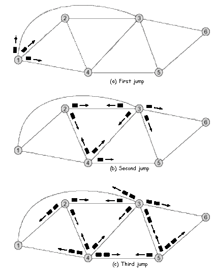
Flood

Routing random

A node selects a single outbound path to retransmit an incoming packet. Selection can be done randomly or alternately

An improvement is that you can select the output path in accordance with the calculation of probabilities

You do not need to use information about the network. In general, the route will not correspond to the one with the least cost or the one with the fewest number of jumps. It has less traffic than Flooding but is equally simple and robust. A node selects a single outgoing path to retransmit an incoming packet. Selection can be done randomly or alternately

An improvement is that you can select the output path in accordance with the calculation of probabilities

You do not need to use information about the network. In general, the route will not correspond to the one with the least cost or the one with the fewest number of jumps. It has less traffic than the flood one but is equally simple and robust

Routing adaptable

Virtually all packet-switched networks used some kind of technique of transmission adaptive

Routing decisions change as network conditions change:

  • Failures
  • Congestion

It requires information about the state of the network presenting disadvantages:

  • Decisions are more complex: higher processing cost at network nodes
  • It is necessary for the nodes to exchange information about the status and traffic of the network: increased traffic and degradation of network performance
  • The reaction too quickly can cause oscillation or be too slow to be relevant

Advantages of routing adaptive

    • Improvement of the performance
    • It is helpful in the control of the congestion
    • Complex system: Theoretical benefits may not be met

Classification

Classification made in accordance with the source of the information

      • Local (isolated)
        • Route the packet to the output link with the tail shorter
        • You can include a weight for each destination. They are rarely used, since they do not easily exploit the information available
      • Adjacent nodes
      • All nodes

Example of routing adaptive isolated
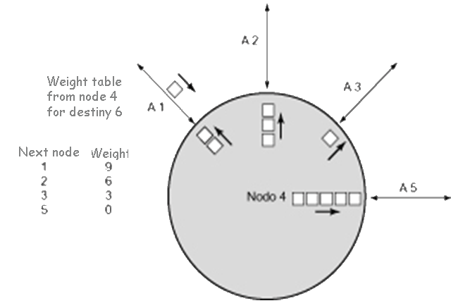
Isolated Adaptive Routing Example

Petri

Petri

A Petri net is a mathematical or graphic representation of a discrete event system in which the topology of a distributed, parallel or concurrent system can be described

The essential Petri net was defined in the 1960s by Carl Adam Petri

They are a generalization of automata theory which allows to express a system of events concurrent

A Petri net is made up of places, transitions, directed arcs and marks or tokens that occupy positions within the places

The rules are: Arches connect a place to a transition as well as a transition to a place

There can be arcs between places or between transitions

The sites contain a finite number or countable infinity of marks

Transitions are triggered, that is, they consume marks from a start position and produce marks at an end position. A transition is enabled if it has marks at all its input positions

In its most basic form, the marks that circulate in a Petri net are all identical

A variant of Petri nets can be defined in which the marks can have a color (information that distinguishes them), an activation time and a hierarchy in the network

Most of the problems on Petri nets are decidable, such as the limited nature and the coverage

To solve them, a Karp-Miller tree is used. The scope problem is known to be decidable, at least in exponential time

Useful in the qualitative analysis

Petri nets can be used to perform the qualitative analysis of a network, since they are bipartite graphs

Depending on how we analyze the Petri net, we can find:

  • Structural analysis (depend on the structure)
    They have the following properties:

    • Repetitive
      There is a sequence of shots, including all transitions, that if they can be triggered leave the system the same as at the beginning \Longleftrightarrow There is a vector that is null right of the matrix of incidence with all its terms positive integers
    • Conservative
      There is a combination of positive integer weights that if applied to the places, the sum of the marking of all the places weighted by their weights is invariant (always the same) \Longleftrightarrow There exists a vector null left of the matrix of incidence with all its terms positive integers
    • Locks
      Place or set of places in which the marks they contain cannot diminish, because the exit transitions of those places are also entrance, with greater total weight in the entrance arches (to the places of the trap) than the output. A row or sum of rows with negative or zero values in the incidence matrix, will contain a lock
    • Traps
      Place or set of places where the marks they contain cannot increase, because the entry transitions to those places are also exiting, with greater total weight in the exit arches (of the trap places) than the input. A row or sum of rows with positive or zero values in the incidence matrix, will contain a trap
    • Lock / Trap
      It is both a lock and a trap. A row or sum of rows with all zero values in the incidence matrix, will contain a lock / trap
  • Dynamic analysis (depend on the initial markup)
    They have the following properties:

    • Cyclic
      Given an initial state, from any accessible state you can always return to the initial state
    • Live
      Given an initial state, from any accessible state there will never be a transition that can no longer be triggered later
    • Limited
      All places have an upper bound finite

The Simplex Method

The Simplex Method

The Simplex method can be used to solve problems of maximizing or minimizing a linear function of variables, with constraints in the form of equalities or inequalities of linear functions of those variables, and with all variables dimensioned above or below

Applying the following steps:

  1. Statement of the problem in standard form
  2. Application of the Simplex algorithm
  3. Determination of the solution obtained

Step 1: Approach the problem as standard

  1. The function should be set to "minimize"
  2. If necessary, variable changes are made so that all variables have 0 as the lower dimension (X_i\geq 0, \forall i)
  3. The restrictions are put with the constant term positive
  4. Become the inequalities of the constraints into equalities by adding the slack variables
  5. Artificial variables are added to constraints that do not have a variable at the base, and the sum of those artificial variables multiplied by M (which is considered with a very high value) is added to the target function.
  6. The table is populated to apply the Simplex algorithm. Its structure is as follows:
    X_1 \cdots X_n
    X basic to b
    c-z

    X_1 \cdots X_n is the alignment of the original variables, slack variables and artificial variables

    to are the terms of such variables in the constraints

    b are the constant elements of such constraints (on the other side of variables in equality)

    c - z are marginal costs, where c are the coefficients of the target function, and z_i=c_{b_1}\cdot a_{1 j}+\cdots+c_{b_m}\cdot a_{m i}, with m being the number of constraints (of elements at the base), and where c_{b_j} represents the coefficient of the target function corresponding to the variable j-th of which they make up the base. Notice that c - z = 0 always for the variables of the base

Step 2: Applying the Simplex Algorithm

  1. Election of the column of pivot
    Looking for the lowest element of the row c - z, c\cdot k - z\cdot k among those who are negative and have a positive element in the column a_k. If there is none the algorithm is terminated
  2. Choice of the row of pivot
    Among the positive elements of a_k looking for the one with the minimum coefficient: \frac{b_i}{a_{i k}}, we'll call it a_{r k}, and that will be the element on which we will pivot. If there are several with the same coefficient you choose any one
  3. Gaussian elimination
    It pivots on a_{r k}, that is, it becomes a_k in a vector of the canonical base. To do this, first divide all the terms in row r from a to a_{r k}, so the new a_{r k} will have a value of 1 (by dividing it between itself). The other elements of the a_k Gaussian elimination (to each i row, with i \not= r, are added the new row r multiplied by X_k). With this the variable -a_{i k} entered the base (and will be located in row r)
  4. Repeat
    Until (c_j - z_j\geq 0, \forall j) \cup (a_k < 0, \forall k\longrightarrow c_k - z_k < 0)

Step 3: Determining the solution obtained

If the problem has artificial variables and some of them have nonzero value in the final solution, then the problem raised has no solution (not feasible). Otherwise, move on to the following cases:

  1. If (c_j - z_j\geq 0, \forall j) \cap (c_k - z_ k > 0) for the variables not basic then we have unique solution
  2. If (c_j - z_j\geq 0, \forall j) \cap (c_k - z_k = 0) for any variable is not basic then we have multiple solutions
  3. If \exists (c_k - z_k < 0) (all of them must comply that a_k < 0) then we have an unstepped solution

Simplex method solutions

Example of problem of the Simplex Method

Example of problem simplex method

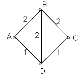
The chart shows the representation of a communication network in which each segment represents the maximum capacity of transfer per unit of time

It is requested to:

  1. It proposes a PPL (linear programming problem) whose solution gives us the maximum transfer capacity between A and B and between C and D (the sum of both)
  2. Solve the PPL (linear programming problem), indicating the type of solution it is, its value, if there is a solution, and explain it

Part a)

Between A and B there are 3 paths that are:

\begin{cases} X_1 \text{ by the way }A-B \\ X_2 \text{ by the way }A-D-B \\ X_3 \text{ by the way }A-D-C-B \end{cases}

Between C and D there are 3 paths that are:

\begin{cases} X_4 \text{ by the way }C-B-A-D \\ X_5 \text{ by the way }C-B-D \\ X_6 \text{ by the way }C-D \end{cases}

Therefore the function to be optimized is:

(X_1+X_2+X_3)+(X_4+X_5+X_6)

With restrictions:

\begin{cases} X_1+X_4 \leq 2 \\ X_2+X_3+X_4 \leq 1 \\ X_3+X_4+X_5 \leq 2 \\ X_2+X_5 \leq 2 \\ X_3+X_6 \leq 1 \end{cases}

With X_1, X_2, X_3, X_4, X_5, X_6 > 0

Part b)

Maximize (X_1+X_2+X_3)+(X_4+X_5+X_6)
Minimize (-X_1-X_2-X_3)+(-X_4-X_5-X_6)

\begin{cases} X_1+X_4+h_1 = 2 \\ X_2+X_3+X_4+h_2 = 1 \\ X_3+X_4+X_5+h_3 = 2 \\ X_2+X_5+h_4 = 2 \\ X_3+X_6+h_5 = 1 \end{cases}

Values c - z:
column \tiny X_1 = -1 - ( (-1) \cdot 1 + 0 \cdot 0 + 0 \cdot 0 + 0 \cdot 0 + (-1) \cdot 0 ) = 0
column \tiny X_2 = -1 - ( (-1) \cdot 0 + 0 \cdot 1 + 0 \cdot 0 + 0 \cdot 1 + (-1) \cdot 0 ) = -1
column \tiny X_3 = -1 - ( (-1) \cdot 0 + 0 \cdot 1 + 0 \cdot 1 + 0 \cdot 0 + (-1) \cdot 1 ) = 0
column \tiny X_4 = -1 - ( (-1) \cdot 1 + 0 \cdot 1 + 0 \cdot 1 + 0 \cdot 0 + (-1) \cdot 0 ) = 0
column \tiny X_5 = -1 - ( (-1) \cdot 0 + 0 \cdot 0 + 0 \cdot 1 + 0 \cdot 1 + (-1) \cdot 0 ) = -1
column \tiny X_6 = -1 - ( (-1) \cdot 0 + 0 \cdot 0 + 0 \cdot 0 + 0 \cdot 0 + (-1) \cdot 1 ) = 0
column \tiny h_1 = 0 - ( (-1) \cdot 1 + 0 \cdot 0 + 0 \cdot 0 + 0 \cdot 0 + (-1) \cdot 0 ) = 1
column \tiny h_2 = 0 - ( (-1) \cdot 0 + 0 \cdot 1+ 0 \cdot 0 + 0 \cdot 0 + (-1) \cdot 0 ) = 0
column \tiny h3 = 0 - ( (-1) \cdot 0 + 0 \cdot 0 + 0 \cdot 1 + 0 \cdot 0 + (-1) \cdot 0 ) = 0
column \tiny h4 = 0 - ( (-1) \cdot 0 + 0 \cdot 0 + 0 \cdot 0 + 0 \cdot 1 + (-1) \cdot 0 ) = 0
column \tiny h5 = 0 - ( (-1) \cdot 0 + 0 \cdot 0 + 0 \cdot 0 + 0 \cdot 0 + (-1) \cdot 1 ) = 1

\tiny{\begin{pmatrix}& -1\hspace{1 mm} X_1& -1\hspace{1 mm} X_2& -1\hspace{1 mm} X_3& -1\hspace{1 mm} X_4& -1\hspace{1 mm} X_5& -1\hspace{1 mm} X_6& 0\hspace{1 mm} h_1& 0\hspace{1 mm} h_2& 0\hspace{1 mm} h_3& 0\hspace{1 mm} h_4& 0\hspace{1 mm} h_5& \cr -1\hspace{1 mm} X_1& 1& 0& 0& 1& 0& 0& 1& 0& 0& 0& 0& 2 \cr 0\hspace{1 mm} h_2& 0& 1& 1& 1& 0& 0& 0& 1& 0& 0& 0& 1 \cr 0\hspace{1 mm} h_3& 0& 0& 1& 1& 1& 0& 0& 0& 1& 0& 0& 2 \cr 0\hspace{1 mm} h_4& 0& 1& 0& 0& 1& 0& 0& 0& 0& 1& 0& 2 \cr -1\hspace{1 mm} X_6& 0& 0& 1& 0& 0& 1& 0& 0& 0& 0& 1& 1 \cr & 0& -1& 0& 0& -1& 0& 1& 0& 0& 0& 1&\end{pmatrix}}

We chose row 2, column 2, as pivot. So in this case \frac{b_i}{a_{i k}} it will be \frac{1}{1}=1

\tiny{\begin{pmatrix}& -1\hspace{1 mm} X_1& -1\hspace{1 mm} X_2& -1\hspace{1 mm} X_3& -1\hspace{1 mm} X_4& -1\hspace{1 mm} X_5& -1\hspace{1 mm} X_6& 0\hspace{1 mm} h_1& 0\hspace{1 mm} h_2& 0\hspace{1 mm} h_3& 0\hspace{1 mm} h_4& 0\hspace{1 mm} h_5& \cr -1\hspace{1 mm} X_1& 1& 0& 0& 1& 0& 0& 1& 0& 0& 0& 0& 2 \cr 0\hspace{1 mm} X_2& 0& 1& 1& 1& 0& 0& 0& 1& 0& 0& 0& 1 \cr 0\hspace{1 mm} h_3& 0& 0& 1& 1& 1& 0& 0& 0& 1& 0& 0& 2 \cr 0\hspace{1 mm} h_4& 0& 0& -1& -1& 1& 0& 0& -1& 0& 1& 0& 1 \cr -1\hspace{1 mm} X_6& 0& 0& 1& 0& 0& 1& 0& 0& 0& 0& 1& 1 \cr & 0& 0& 1& 1& -1& 0& 1& 1& 0& 0& -1& 1\end{pmatrix}}

We chose row 4, column 5, as pivot. So in this case \frac{b_i}{a_{i k}} it will be \frac{1}{1}=1

\tiny{\begin{pmatrix}& -1\hspace{1 mm} X_1& -1\hspace{1 mm} X_2& -1\hspace{1 mm} X_3& -1\hspace{1 mm} X_4& -1\hspace{1 mm} X_5& -1\hspace{1 mm} X_6& 0\hspace{1 mm} h_1& 0\hspace{1 mm} h_2& 0\hspace{1 mm} h_3& 0\hspace{1 mm} h_4& 0\hspace{1 mm} h_5& \cr -1\hspace{1 mm} X_1& 1& 0& 0& 1& 0& 0& 1& 0& 0& 0& 0& 2 \cr 0\hspace{1 mm} h_2& 0& 1& 1& 1& 0& 0& 0& 1& 0& 0& 0& 1 \cr 0\hspace{1 mm} h_3& 0& 0& 2& 2& 0& 0& 0& 1& 1& -1& 0& 1 \cr 0\hspace{1 mm} X_5& 0& 0& -1& -1& 1& 0& 0& -1& 0& 1& 0& 1 \cr -1\hspace{1 mm} X_6& 0& 0& 1& 0& 0& 1& 0& 0& 0& 0& 1& 1 \cr & 0& 0& 0& 0& 0& 0& 1& 0& 0& 1& -1& 2\end{pmatrix}}

Since there are no more negative values in c – z, c_k - z_k that we can pivot, we stop the algorithm and we get the following result:

\begin{cases} X_1 = 2 \\ X_2 = 1 \\ X_5 = 1 \\ X_6 = 1 \end{cases}

Therefore, we have to X_3 = 0 and X_4 = 0 to enforce the restrictions. So we have a possible solution to our problem is:

(X_1+X_2+X_3)+(X_4+X_5+X_6) = 5

The solution is multiple, therefore, this solution is not the only

Algorithm Bellman-Ford

Algorithm Bellman-Ford

The algorithm Bellman-Ford solves the problems in which there is to find the shortest paths from a source node given with the condition that they contain at most one link

Find the shortest paths with the condition of containing two links maximum

And so on until the maximum number of shortest paths

Where:

  • s = source node
  • w(i, j) = link cost from node i to node j:
    • w(i, i) = 0
    • w(i, j) = \infty if the two nodes are not directly connected
    • w(i, j) \geq 0 if the two nodes are directly connected
  • h = maximum number of links in a path in the current step of the algorithm
  • L_h(n) = cost of the path of minimum cost from the node s to the node n with the condition that there is no more than h links

For resolution you can use the Bellman-Ford algorithm method, which consists of applying the following steps:

  1. Initialization
  2. Update

Step 1: Initialization

L_0(n) = \infty, \forall n \not= s
L_h(n) = 0, \forall h

Step 2: Update

  1. For each successive h \geq 0, \forall n \not= s calculate:
    L_{h+1}(s)=\min_j{[L_h(j)+w(j, n)]}
  2. Connect n with the node predecessor j of minimum cost
  3. Remove all connections of n with a node predecessor different obtained in a previous iteration
  4. The path from s to n terminates with link from j to n

Annotations to the algorithm, Bellman-Ford

For the iteration of step 2 with h'K, and for each target node n, the algorithm compares the potential paths of length K + 1 from s to n with the existing path at the end of the previous iteration

If the shortest path before has a lower cost, it is saved

Otherwise, a new path is defined

Example of algorithm Bellman-Ford

Example of algorithm Bellman-Ford

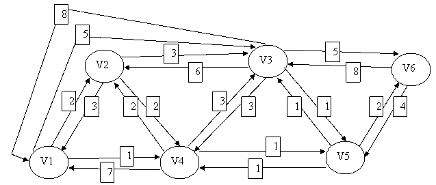
The chart shows the representation of a communication network in which each segment represents the maximum capacity of transfer per unit of time

It is requested to:

To get from node V1 to node V6

h L_h(2) Route L_h(3) Route L_h(4) Route L_h(5) Route L_h(6) Route
0 \infty \infty \infty \infty \infty
1 2 1-2 5 1-3 1 1-4 \infty \infty
2 2 1-2 4 1-4-3 1 1-4 2 1-4-5 10 1-3-6
3 2 1-2 3 1-4-5-3 1 1-4 2 1-4-5 4 1-4-5-6
4 2 1-2 3 1-4-5-3 1 1-4 2 1-4-5 4 1-4-5-6

According to the Bellman-Ford algorithm we will have to follow the V1-V4-V5-V6 nodes, because they are the ones that cause the least cost

Algorithm Dijkstra

Algorithm Dijkstra

The Dijkstra algorithm solves the problems in which the shortest paths between a given source node and all other nodes need to be found, developing the paths in increasing order of length

Where:

  • N = set of nodes in the network
  • s = source node
  • T = list or set of nodes added to, or incorporated by the algorithm
  • w(i, j) = link cost from node i to node j:
    • w(i, i) = 0
    • w(i, j) = \infty if the two nodes are not directly connected
    • w(i, j) \geq 0 if the two nodes are directly connected
  • L_h(n) = cost, of course, obtained by the algorithm for the path of minimum cost from node s to node n

For resolution you can use the Dijkstra algorithm method, which consists of applying the following steps:

  1. Initialization
  2. Getting the next node
  3. Update the paths of minimum cost

Step 1: Initialization

T = {s} the built-in node set only consists of the source node

L(n) = w(s, n), \forall n \not= s

The initial cost of the routes to the neighboring nodes is associated to the links

Step 2: Getting the next node

  1. Looking to the neighbouring node that is not in T with the path of least cost
  2. It incorporates the node in T
  3. It incorporates the link from that node to a node of T that is part of the way

Step 3: Updating the Minimum Cost Roads

The following formula applies:

L(n) = \min{[L(n), L(x) + w(x, n)]}, \forall n \not\in T

The algorithm concludes when all nodes have been added to T

Annotations to the algorithm Dijkstra

In the end, the L(x) value associated with each x node is the cost (length) of the minimum cost path from s to x

T defines the path of minimum cost from s to any other node

Each iteration of steps 2 and 3 incorporates a new node to T that defines the minimum cost path from s to that node, traversing that path only nodes included in T

Example of the algorithm Dijkstra

Example of the algorithm Dijkstra

The chart shows the representation of a communication network in which each segment represents the maximum capacity of transfer per unit of time

It is requested to:

To get from node V1 to node V6

i T L_h(2) Route L_h(3) Route L_h(4) Route L_h(5) Route L_h(6) Route
1 {1} 2 1-2 5 1-3 1 1-4 \infty \infty
2 {1, 4} 2 1-2 4 1-4-3 1 1-4 2 1-4-5 \infty
3 {1, 2, 4} 2 1-2 4 1-4-3 1 1-4 2 1-4-5 \infty
4 {1, 2, 4, 5} 2 1-2 3 1-4-5-3 1 1-4 2 1-4-5 4 1-4-5–6
5 {1, 2, 3, 4, 5} 2 1-2 3 1-4-5-3 1 1-4 2 1-4-5 4 1-4-5–6
6 {1, 2, 3, 4, 5, 6} 2 1-2 3 1-4-5-3 1 1-4 2 1-4-5 4 1-4-5–6

According to the Dijkstra algorithm we will have to follow the V1-V4-V5-V6 nodes, because they are the ones that cause the least cost